Exercise 9M2

For exercise 9M2, the question is ambiguous, about whether you should use the original dexp(1) or the dunif(0,1) from 9M1 as the prior for sigma. Use dexp(1) and only change the prior for b from the m9.1 in the book.

Exercises 9M1–9M2

For comparing the results, you should both look at the precis of the models and also plot the densities of the posteriors.

To easily plot the densities of the posteriors for one model, do the following (assume the model from the book is m9.1, and the models from the exercises are ex9m1 and ex9m2).

This is equivalent to the code from the textbook for m9.1:

library(cmdstanr)
library(rethinking)
library(tidyverse)

data(rugged)
d <- rugged %>% mutate(log_gdp = log(rgdppc_2000))

dd <- d %>% filter(complete.cases(rgdppc_2000)) %>%
  mutate(
    log_gdp_std = log_gdp / mean(log_gdp),
    rugged_std = rugged / max(rugged),
    cid = ifelse(cont_africa == 1, 1, 2)
  )

dat_slim <- dd %>% select(log_gdp_std, rugged_std, cid) %>%
  mutate(cid = as.integer(cid))

m9.1 <- ulam(
  alist(
    log_gdp_std ~ dnorm(mu, sigma),
    mu <- a[cid] + b[cid] * (rugged_std - 0.215) ,
    a[cid] ~ dnorm(1, 0.1),
    b[cid] ~ dnorm(0, 0.3),
    sigma ~ dexp(1)
  ), data=dat_slim, chains = 4, cores = 4, cmdstan = TRUE)

This code will plot the posterior probability densities:

library(tidybayes)
library(tidybayes.rethinking)
library(bayesplot)

draws <- tidy_draws(m9.1)
mcmc_dens(draws)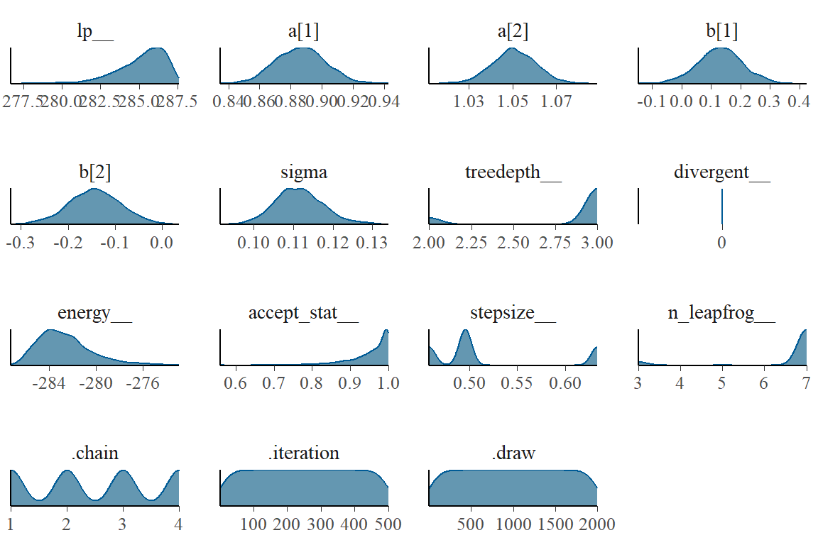

If you have two models, foo and bar, you can compare the posteriors of a parameter like sigma using code like this, from the textbook:

post_foo <- extract.samples(foo)
post_bar <- extract.samples(bar)

dens(post_foo$sigma, lwd = 1)
dens(post_bar$sigma, lwd = 1, col = rangi2, add = TRUE)

Alternately, you can do the same thing using the tidyverse dialect:

foo_draws <- tidy_draws(foo) %>% mutate(model = "foo")
bar_draws <- tidy_draws(bar) %>% mutate(model = "bar")

bind_rows(foo_draws, bar_draws) %>% 
  ggplot(aes(x = sigma, color = model, fill = model)) + 
  geom_density(size = 1, alpha = 0.3)

The first two lines extract the Monte-Carlo samples of the posterior for each model, and add a label model to indicate which model they came from. Then I use ggplot to plot the posterior density of sigma, from each model, where the color of the line and the fill inside the density plot indicate which model is which.

The argument size = 1 tells R how thick to make the line, and alpha = 0.3 sets the transparency of the fills (1 = completely opaque and 0 = completely transparent)

If you want to make a single plot that shows comparisons of all the parameters for both models, the code gets a bit more complicated:

foo_draws <- tidy_draws(foo) %>%
  gather_draws(a[i], b[i], sigma) %>%
  mutate(model = "foo")
bar_draws <- tidy_draws(bar) %>%
  gather_draws(a[i], b[i], sigma) %>%
  mutate(model = "bar")

bind_rows(foo_draws, bar_draws) %>% 
  mutate(.variable = ifelse(is.na(i), .variable,
                            str_c(.variable, "[", i, "]"))) %>%
  ggplot(aes(x = .value, col = model, fill = model)) + 
  geom_density(alpha = 0.3) + labs(x = NULL, y = NULL) + 
  facet_wrap(~.variable, scales = "free")

Exercises 11E1–11E3

To check yourself, for 11E1 the log-odds is -0.619, for 11E2 the probability is 0.961, and for 11E3 the proportional change in the odds is 5.47

Exercise 11M7

For 11M7, I recommend using the following code to compare the precises of the two models (m11.4 is the ulam model on page 330, and m11.4q is the quap version model that you should write for this exercise). This code prints the two precises side-by-side with each row representing a different parameter.

pr <- precis( m11.4 , 2 )[,1:4]
prq <- precis( m11.4q , 2 )
round( cbind( pr , prq ) , 2 )

Then for parameters that are really different in the two models (differences of more than 0.1 in the means or the 5.5% or 94.5% levels), make a density plot comparing the posteriors of the two models. You can use the code from my notes (above) for exercises 9M1 and 9M2 to do this. Think about what important differences you see in the posteriors from the two models, and what I’ve been emphasizing in class about the differences between the quap and Monte-Carlo methods for estimating posteriors.

You can also use the code, above, in the notes for 9M1 and 9M2, to make a single plot comparing the posteriors of all the parameters for both models. Then you can make a single comparison plot for any of the parameters that show significant differences between the quap and ulam models.

At the minimum, be sure to look carefully at a[2].